
One of the core principles of software engineering is “encapsulation”. However, this principle is often overlooked when deploying a machine-learned model. A machine-learned model is a composite of two things: transformations (such as One Hot Encoding, Imputing Values, etc.) and scoring (e.g., Linear Regression). Nevertheless, the serialized model often only contains the model’s scoring part, and transformations are implemented at the application layer.
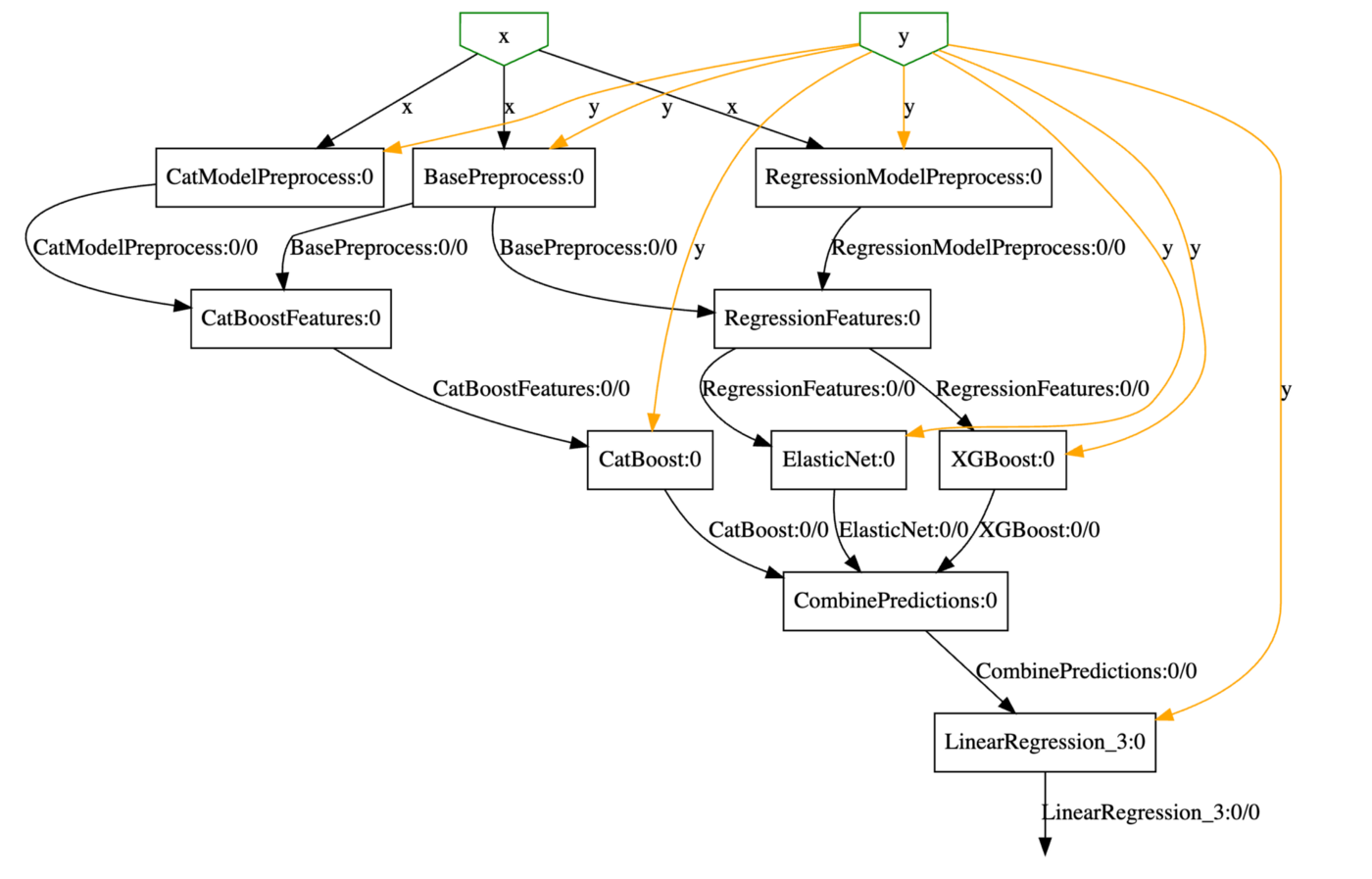
This post shows how both transformations and scoring can be serialized together using sklearn-pandas and baikal. The below diagram represents the architecture of an ensemble model to predict house price. The dataset I used for this model is related to the “house price” competition on Kaggle. First, the grey boxes represent various transformations on the data. For instance, missing data is imputed, categorical data is encoded, etc. Next, I use three different algorithms( ElasticNet, XGBoost, and CatBoost) to generate three independent predictions. The three predictions serve as an input to a simple linear regression algorithm (ensemble model) and serve as the final model.

Full code for training the above DAG is available over here. However, before you go over there, notice some of the advantages of leveraging sklearn-pandas and baikal.
- Generating Predictions: I started the post with the topic of “encapsulation.” The code below demonstrates what I wanted to achieve. Notice that the serialized model hides all the complexity of data processing and stacking. As a consumer of the model, I have a familiar sklearn API; all I need to do is call the “predict” function and pass the raw data.
import pandas as pd
import cloudpickle
# load test data
testDF = pd.read_csv('data/test.csv')
# load serialized model
with open('resources/model.pkl', 'rb') as fp:
    model = cloudpickle.load(fp)
# Generate predictions
model.predict(testDF)
2. Displaying the DAG: The model object is not a black box but can be visualized as well.
from baikal.plot import plot_model
from IPython.display import SVG
plot_model(model, filename='resources/model.svg')
SVG('resources/model.svg')
3. Examining intermediate results: You are not limited to final prediction but intermediate results can also be easily examined. For instance, the code below examines the output of CatBoostFeatures step. This step prepares the data for the consumption of the CatBoost Model. Notice that the output is a data frame with descriptive names; one of the features of sklearn-pandas and the reason I love using it.
output = model.predict(data, output_names=['CatBoostFeatures:0/0'])

Finally, the code block shows how the DAG was constructed using Baikal.
# Define Input and Target Variable
x = Input(name="x")
y = Input(name='y')
# Define Data Processing Steps
d0 = DataFrameMapperStep(baseProcessing, df_out=True, name='BasePreprocess')(x, y)
d1 = DataFrameMapperStep(regressionModelProcessing, df_out=True, name='RegressionModelPreprocess')(x, y)
d2 = DataFrameMapperStep(catModelPreprocessing, df_out=True, name='CatModelPreprocess')(x, y)
# Compose Features
regressionFeatures = ConcatStep(name='RegressionFeatures')([d0, d1])
catFeatures = ConcatStep(name='CatBoostFeatures')([d0, d2])
# Define Independent Models
m1 = ElasticNetStep(name='ElasticNet')(regressionFeatures, y)
m2 = XGBRegressorStep(name='XGBoost')(regressionFeatures, y)
m3 = CatBoostRegressorStep(name='CatBoost', cat_features=CATEGORICAL_COLUMNS, iterations=10)(catFeatures, y)
# Combine predictions into a single dataset
combinedPredictions= Stack(name='CombinePredictions')([m1, m3])
# Create an ensemble model
ensembleModel = LinearRegressionStep()(combinedPredictions, y)
model = Model(x, ensembleModel, y)
# Fit the model
model.fit(data, data['SalePrice'])
# serialize model for deployment
import cloudpickle
with open('resources/model.pkl', 'wb+') as fp:
    cloudpickle.dump(model, fp)
Summary:
- transformations and scoring are two aspects of a machine-learned model and both should be part of any serialized model. You can find the full sample code on how to package the two together over here.
- sklearn-pandas provides a nice interface to manage transformations and since it has the ability to return pandas data frame, it much easier to debug and understand the source of a particular numerical value.
- baikal is a great resource for creating DAG. Unlike sklearn’s pipeline that can only handle linear graphs, baikal can easily handle diamonds and other forms of DAG.
